What is Imposter Syndrome?
Impostor syndrome (also known as impostor phenomenon, fraud syndrome or the impostor experience) is a concept describing individuals who are marked by an inability to internalize their accomplishments and a persistent fear of being exposed as a “fraud”
What brought me to blog / explore about this subject is that, quite often if not everyday I feel like this feeling on being inadequate. I made Twitter my bedtime story. I always get excited to find new things that I potentially can learn and immediately sense of sadness when my self-doubt kicks in - that I am actually not good enough to accompolish it.
Then I came across this tweet:
I feel like every now and then, I look around and people say they feel like they are frauds or rocking some serious #ImposterSyndrome. I see a ton of advice on this topic, but I'm not sure how much of it works for grouches like me.
— Bridget Cogley (@WindsCogley) February 19, 2018
Buddhists also talk about recognizing discomforts, not always correcting them. So, there's that thought as well. https://t.co/JxiPx1bxbp
— Bridget Cogley (@WindsCogley) February 19, 2018
So I am not alone then??
I responded to her tweet. And it occured to me - how do others handle this Imposter Syndrome what are their takes on it?
*Exploing tweets that contain the word “Imposter Sydrome”
## search for 18000 tweets using the rstats hashtag - I totally got this post from one of Emily Robinson's post on RStudio website - Thank you kindly :) - oh I changed the search criteria obviously.

rt <- search_tweets(
  "imposter syndrome", n = 18000, include_rts = FALSE
)

## plot time series of tweets
ts_plot(rt, "3 hours") +
  ggplot2::theme_minimal() +
  ggplot2::theme(plot.title = ggplot2::element_text(face = "bold")) +
  ggplot2::labs(
    x = NULL, y = NULL,
    title = "Frequency of imposter syndrome tweets",
    subtitle = "Twitter status (tweet) counts aggregated using three-hour intervals",
    caption = "\nSource: rtweet package"
  )
rt <- lat_lng(rt)Where are these tweets from?
And this is something effect people everywhere too? Not all tweets are geo-coded….so many really there are more data points.
## Warning in validateCoords(lng, lat, funcName): Data contains 1851 rows with
## either missing or invalid lat/lon values and will be ignored

- I would like to extract more information on tweets so I am going to use “TidyText” package for tokenisation.
## do a bit to tidy with Regex
drop_pattern <- "https://t.co/[A-Za-z\\d]+|http://[A-Za-z\\d]+|&|<|>|RT|https|ht"
unnest_pattern <- "([^A-Za-z_\\d#@']|'(?![A-Za-z_\\d#@]))"
df3 = df2 %>%
mutate(text_clean = stringr::str_replace_all(text, drop_pattern, "")) %>%
unnest_tokens(word,
text,
token = "regex",
pattern = unnest_pattern) %>% anti_join(custom_stop_words)## Joining, by = "word"##word count
df3 %>% count(word, sort = TRUE)## # A tibble: 7,293 x 2
## word n
## <chr> <int>
## 1 syndrome 1875
## 2 imposter 1863
## 3 feel 151
## 4 people 139
## 5 feeling 114
## 6 time 100
## 7 amp 98
## 8 real 94
## 9 beat 92
## 10 person 82
## # ... with 7,283 more rowsSentiment Analysis
##I choose Bing lexico because I want to do a straight comparison between positive / negative sentiment.

bing = get_sentiments("bing")
bing_rt = df3 %>% inner_join(bing) %>%
  count(word, sentiment, sort = TRUE) %>%
  ungroup()
## Joining, by = "word"bing_rt## # A tibble: 808 x 3
## word sentiment n
## <chr> <chr> <int>
## 1 syndrome negative 1875
## 2 hard negative 53
## 3 suffer negative 52
## 4 doubt negative 45
## 5 love positive 41
## 6 confidence positive 40
## 7 struggle negative 37
## 8 fear negative 36
## 9 anxiety negative 32
## 10 bad negative 32
## # ... with 798 more rows##Plot data using ggplot2 for initial explorary analysis - top 10 words for Positive and Negative sentiments.
library(ggplot2)
bing_rt %>%
group_by(sentiment) %>%
top_n(10) %>%
ungroup() %>%
mutate(word = reorder(word, n)) %>%
ggplot(aes(word, n, fill = sentiment)) +
geom_col(show.legend = FALSE) +
facet_wrap(~sentiment, scales = "free_y") +
labs(y = "Contribution to sentiment",
x = NULL) +
coord_flip()## Selecting by n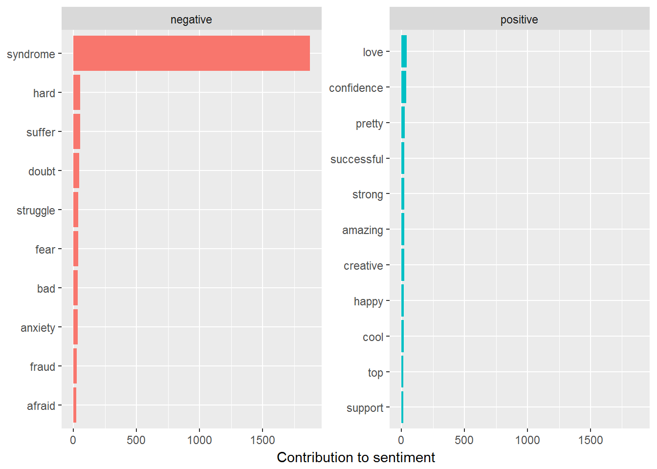
##Can wordcloud give it more distinct visual comparison?

library(reshape2)
##
## Attaching package: 'reshape2'## The following object is masked from 'package:tidyr':
##
## smithslibrary(wordcloud)## Loading required package: RColorBrewerdf3 %>%
inner_join(get_sentiments("bing")) %>%
count(word, sentiment, sort = TRUE) %>%
acast(word ~ sentiment, value.var = "n", fill = 0) %>%
comparison.cloud(colors = c("gray20", "gray80"),
max.words = 100)## Joining, by = "word"
What are things that mentioned in the context of Imposter Syndrome? I use “widyr” to help me explore it further.
word_pairs <- df3 %>%
  pairwise_count(word, id, sort = TRUE, upper = FALSE)

word_pairs
## # A tibble: 95,804 x 3
## item1 item2 n
## <chr> <chr> <dbl>
## 1 imposter syndrome 1786
## 2 imposter feel 127
## 3 syndrome feel 126
## 4 imposter people 120
## 5 syndrome people 120
## 6 imposter feeling 100
## 7 syndrome feeling 99.0
## 8 syndrome beat 90.0
## 9 imposter real 86.0
## 10 syndrome real 86.0
## # ... with 95,794 more rowsset.seed(1234)
word_pairs %>%
filter(n >= 30) %>%
graph_from_data_frame() %>%
ggraph(layout = "fr") +
geom_edge_link(aes(edge_alpha = n, edge_width = n), edge_colour = "cyan4") +
geom_node_point(size = 5) +
geom_node_text(aes(label = name), repel = TRUE,
point.padding = unit(0.2, "lines")) +
theme_void()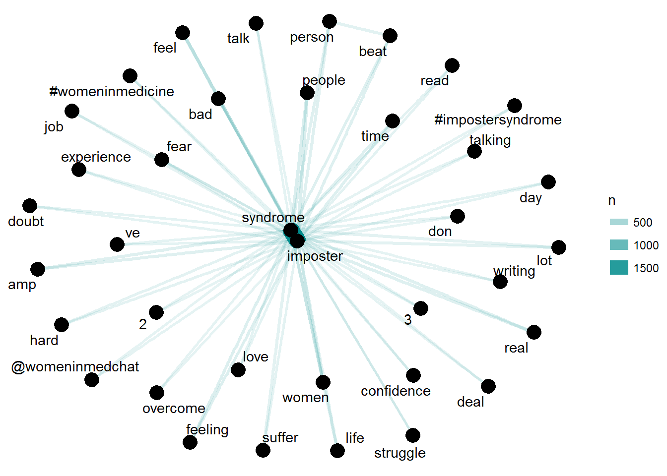
Conclusion
I understand that how I feel isnt unique to me and a lot of people also are reaching out for supports. Self-compassion is important too. As one of favourite authors Jack Kornfield says
“If your compassion does not include yourself, it is incomplete.”

Caption for the picture.